The Math Behind the Magic: My Neural Networks & Deep Learning Journey at GWU

I'm currently pursuing my MS in Computer Science at George Washington University, and this semester I enrolled in CSCI 6366: Neural Networks & Deep Learning taught by Professor John Sipple. Before walking into this class, I had built ML projects — fraud detection systems, LSTM-based weather forecasters, sentiment analysis pipelines. I thought I understood deep learning.

Turns out, I understood how to use deep learning. I didn't fully understand how it works.

This blog is my attempt to document what I've learned so far — not as a textbook summary, but as an honest account of the concepts that clicked, the ones that challenged me, and the insights I wish someone had told me earlier.

Why This Course Hit Different

Most online tutorials teach you to model.fit() and call it a day. This course does the opposite. In the very first lecture, Professor Sipple laid out the philosophy: you need to understand the math, the theory, and the intuition before you touch a framework.

That means before writing a single line of PyTorch, we spent weeks on linear algebra, calculus, probability, and information theory. At first, I'll admit — I wondered why. I already knew what a matrix was. I'd done gradient descent in my head a hundred times.

But here's what I realized: there's a massive gap between recognizing a concept and understanding it deeply enough to debug a failing model at 2 AM.

The Foundations Nobody Talks About

Linear Algebra — It's Not Just Matrix Multiplication

Everyone knows neural networks use matrices. But the course forced me to think about why. A few things that shifted my perspective:

Eigendecomposition isn't abstract math — it tells you about your model's behavior. When you decompose a matrix into its eigenvalues and eigenvectors, you're essentially asking: "In which directions does this transformation stretch or compress?" In deep learning, this directly relates to how gradients flow through your network. If your weight matrix has eigenvalues much greater or less than 1, you're looking at exploding or vanishing gradients — before you even start training.

SVD is everywhere. Singular Value Decomposition isn't just a linear algebra concept — it shows up in dimensionality reduction, in understanding how your network compresses information, and even in modern techniques like LoRA for fine-tuning LLMs. The key insight: any matrix, even non-square ones, can be decomposed into rotation, scaling, and another rotation. That's essentially what every layer of your network is doing.

The condition number tells you if your problem is cursed. A matrix with a high condition number means your system is numerically unstable — small input changes lead to wildly different outputs. When I connected this to the instability I'd seen in some of my own regression models, it clicked. The math wasn't abstract; it was a diagnostic tool.

Calculus — Gradients Are Your GPS

I knew derivatives before this course. What I didn't appreciate was the full picture of optimization geometry.

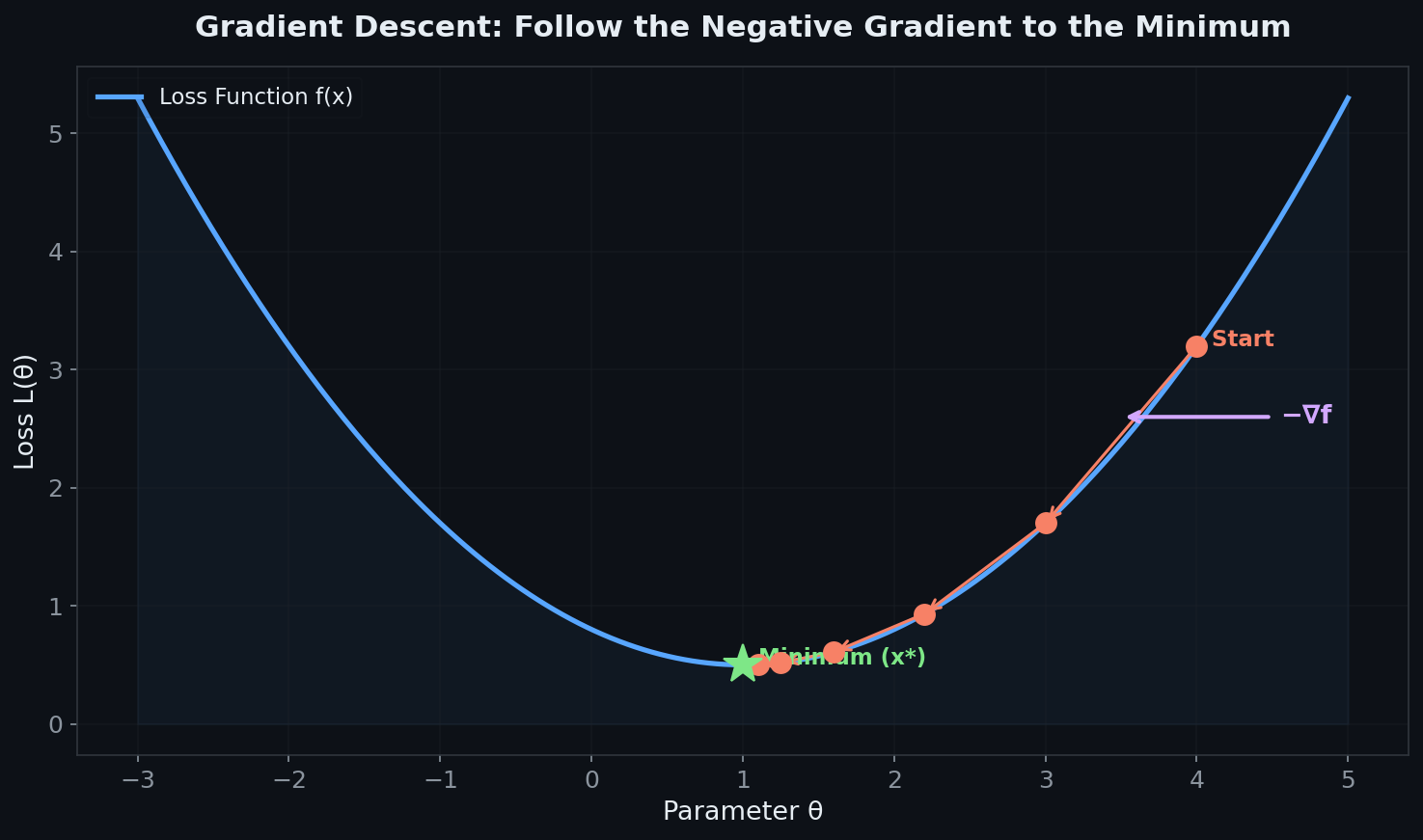
The gradient isn't just a slope — it's a direction. In high-dimensional spaces (which is basically every neural network), the gradient tells you which direction to move to reduce loss the fastest. The formula is elegant: to minimize a function, walk in the opposite direction of its gradient. That's literally all gradient descent is.

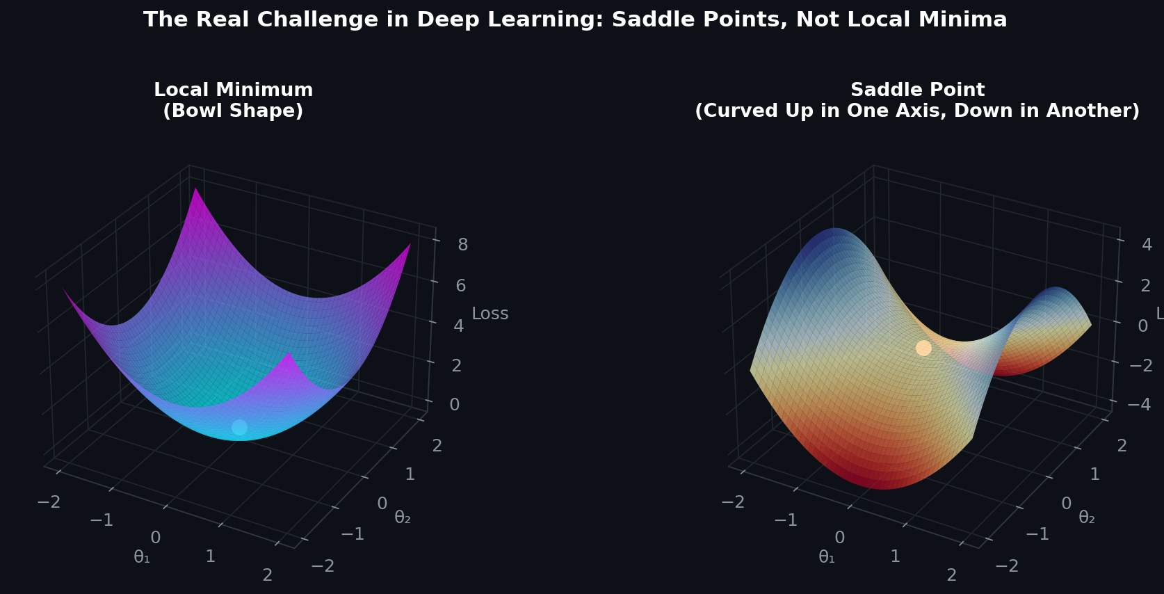
The Hessian reveals the curvature of your loss landscape. The first derivative tells you the slope. The second derivative (the Hessian matrix) tells you the shape — are you in a bowl (good, a minimum), sitting on a hilltop (bad, a maximum), or on a saddle point (tricky, common in high dimensions)?

Here's a key insight from lecture: saddle points, not local minima, are the real challenge in deep learning. In high-dimensional spaces, true local minima are rare. Most critical points are saddle points — flat in some directions, curved in others. This is why SGD with momentum works: it has enough "velocity" to escape saddle points that pure gradient descent would get stuck on.

The Taylor series approximation is the secret behind nearly every optimization algorithm. When you approximate a function using its first and second derivatives, you get the foundation for Newton's method, BFGS, and even the intuition behind learning rate schedules. The second-order term tells you how much to "trust" the gradient — if the curvature is high, you should take smaller steps.

Probability & Information Theory — The Language of Learning

This section was genuinely eye-opening for me. I'd used cross-entropy loss hundreds of times without deeply understanding why it works.

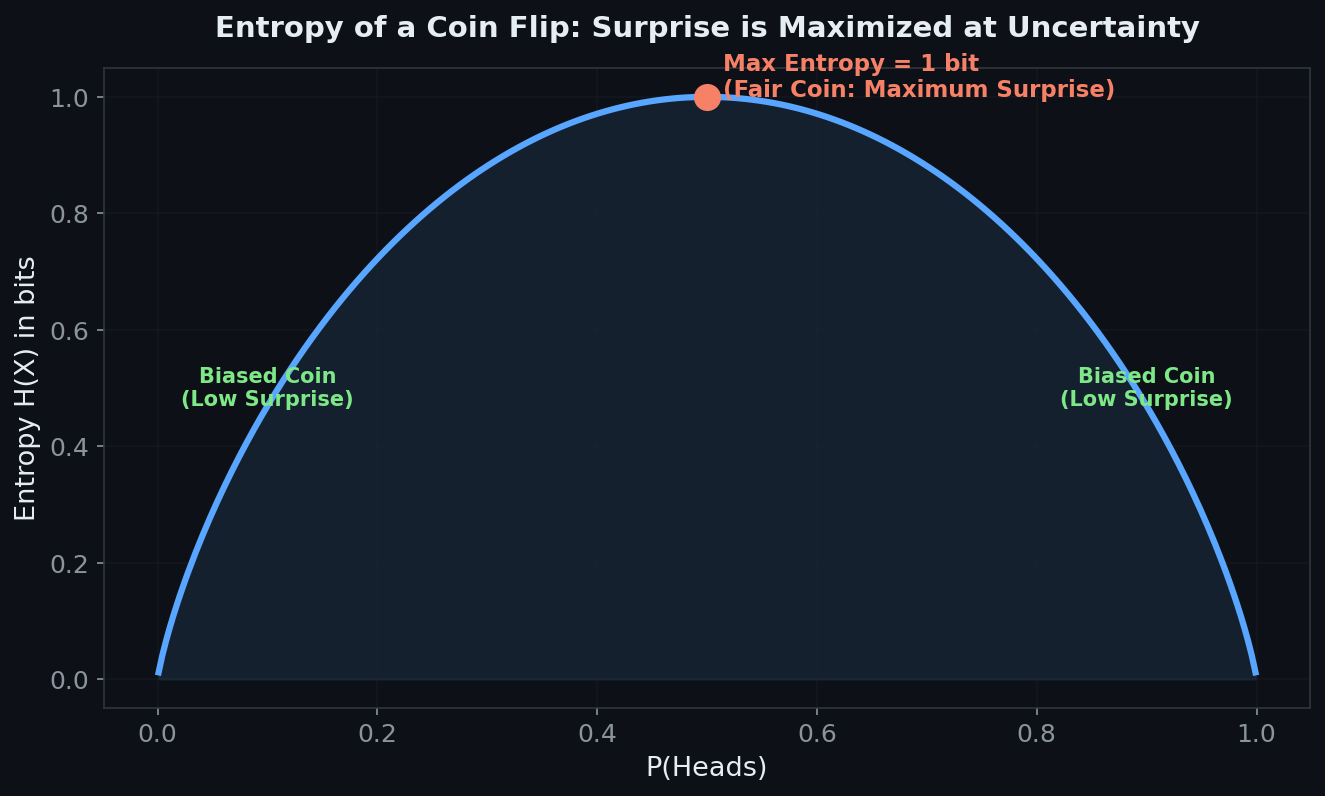
Entropy measures surprise, not randomness. A fair coin has maximum entropy (1 bit) — each flip is maximally surprising. A biased coin (say, 99% heads) has low entropy — you're rarely surprised. In ML, we want our model's predicted distribution to have low entropy relative to the true distribution. That's what training does: it reduces the model's "surprise."

Cross-entropy loss connects directly to KL divergence. Minimizing cross-entropy between your predicted distribution and the true label distribution is equivalent to minimizing KL divergence plus the entropy of the true distribution. Since the entropy of the true labels is fixed, minimizing cross-entropy is minimizing KL divergence. This means when you train a classifier with cross-entropy loss, you're literally asking: "How can I make my predicted distribution as close as possible to the true distribution?"

KL divergence is asymmetric, and that matters. D_KL(P || Q) ≠ D_KL(Q || P). When we minimize D_KL(P || Q) where P is the true distribution, we're saying "wherever P puts probability mass, Q better put mass there too." This means the model learns to cover all modes of the true distribution rather than just capturing the most prominent mode. This asymmetry has practical implications in generative models (like VAEs) where the direction of KL divergence determines whether you get mode-covering or mode-seeking behavior.

Optimal Transport offers a geometric alternative. One concept that surprised me was the Earth Mover's Distance — instead of measuring "coding inefficiency" like KL divergence, it asks: "What's the minimum cost to transform one distribution into another?" This is especially powerful when distributions have disjoint support (no overlap), where KL divergence just blows up to infinity but EMD gives a meaningful, finite distance. This is why Wasserstein GANs use EMD — it provides useful gradients even when the generator's distribution doesn't overlap with the real data.

The Learning Paradigm — A Framework for Everything

One of the most clarifying moments in the course was when Professor Sipple presented the general learning paradigm. Every supervised deep learning algorithm, at its core, follows three steps:

1. Define a loss function — How do you measure how wrong your model is?

2. Derive the gradient — How does the loss change when you tweak each parameter?

3. Optimize — Either solve for the minimum analytically (rare) or iteratively update parameters using gradient descent.

Show Image

Once I internalized this framework, everything from linear regression to massive transformer models became variations on the same theme. The differences are in the architecture (how you parameterize your model), the loss function (what you're optimizing for), and the optimizer (how you navigate the loss landscape). But the paradigm? Always the same.

Linear Models — Simple but Revealing

Regression: The Closed-Form Solution

Linear regression was our first "model." The beautiful thing about it: you can solve it analytically. Set the derivative of L2 loss to zero, and you get the normal equation. No iterative optimization needed.

But here's what I found insightful — the closed-form solution reveals exactly when linear regression breaks. If your feature matrix isn't full rank, the inverse doesn't exist. If features are nearly collinear, the condition number explodes and your solution becomes numerically unstable. Small perturbations in input lead to dramatic changes in predictions.

This is exactly where regularization enters the picture, not as an afterthought but as a mathematical necessity.

Ridge vs. Lasso — A Tale of Two Penalties

Ridge regression (L2) adds a penalty proportional to the squared magnitude of weights. This shrinks all coefficients toward zero but never exactly to zero. The resulting closed-form solution adds λI to the matrix before inversion — essentially making the system more stable by construction.

Lasso regression (L1) uses the absolute value of weights as the penalty. Unlike Ridge, it drives some coefficients to exactly zero — effectively performing feature selection. The tradeoff? No closed-form solution; you need iterative optimization.

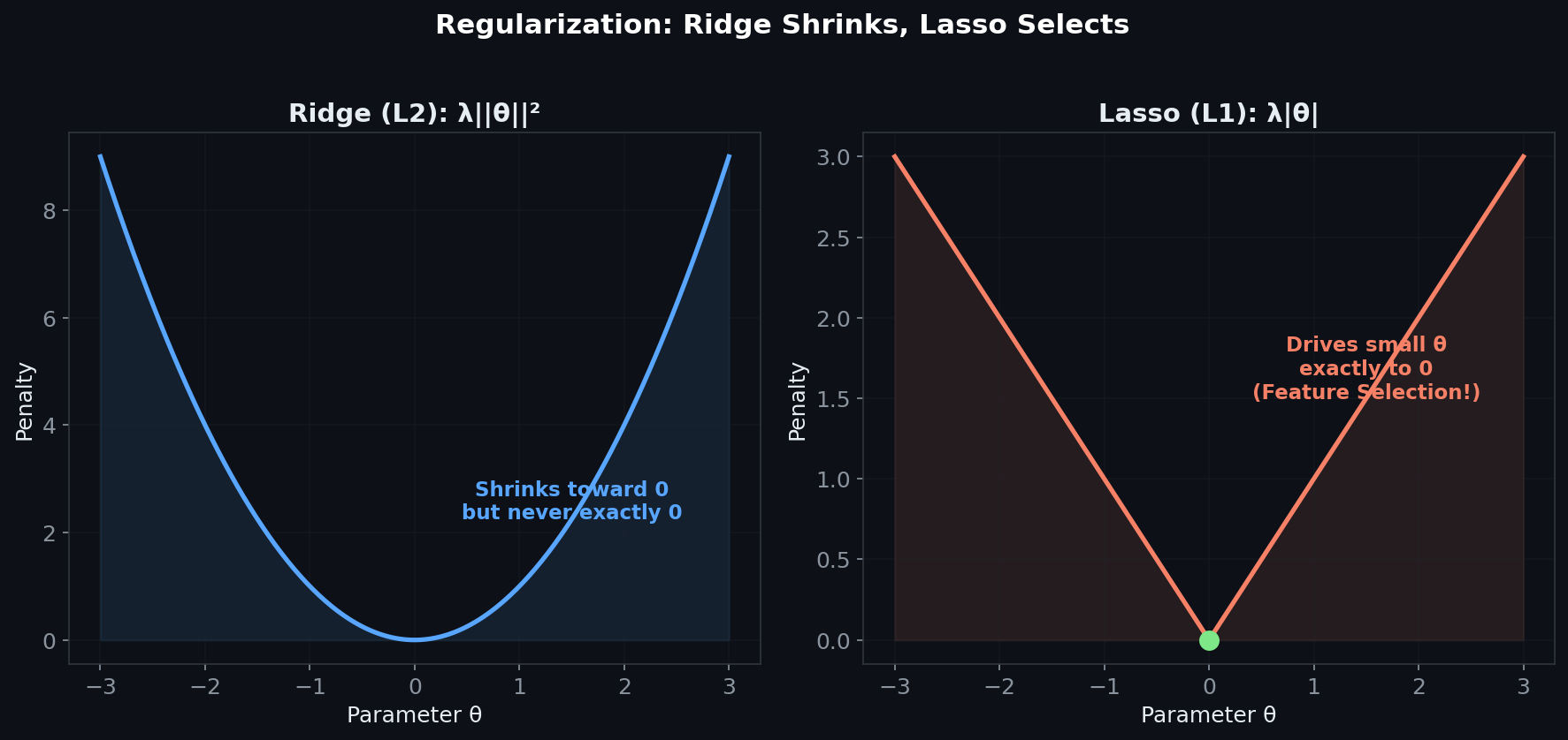
The choice between them isn't arbitrary. If you believe all features contribute a little, use Ridge. If you suspect only a few features matter and want automatic selection, use Lasso. In production ML systems, this distinction directly impacts model interpretability and inference speed.

Classification: Planes, Dot Products, and Probabilities

The way classification was taught in this course gave me a much richer geometric intuition. Instead of jumping straight to logistic regression, we started with the point-normal representation of a plane.

A hyperplane divides your feature space into two halves. For any point, the dot product with the plane's normal vector tells you which side it's on — positive or negative. The sign gives you the class, and the magnitude gives you the confidence.

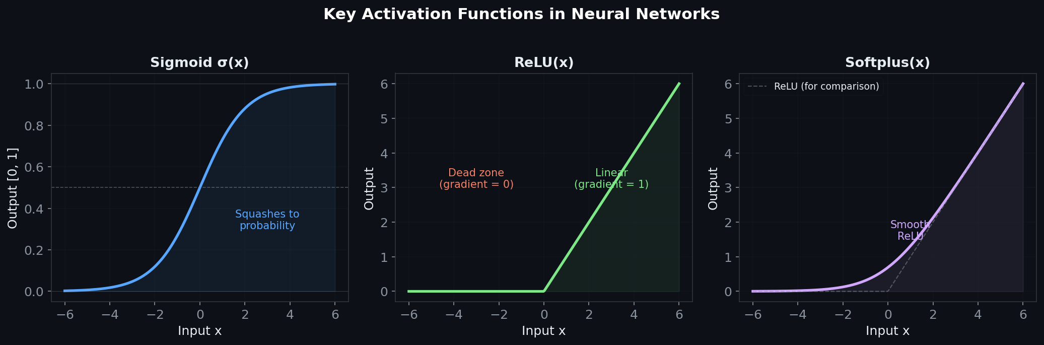
The problem? The dot product ranges from -∞ to +∞, and we need probabilities [0, 1]. Enter the sigmoid function, which squashes any real number into that range. Apply cross-entropy loss, and you've got logistic regression — built up from geometric first principles rather than presented as a magic formula.

For multi-class problems, we extend this to multiple hyperplanes and replace sigmoid with softmax. Each class gets its own hyperplane, and softmax converts the raw scores into a valid probability distribution.

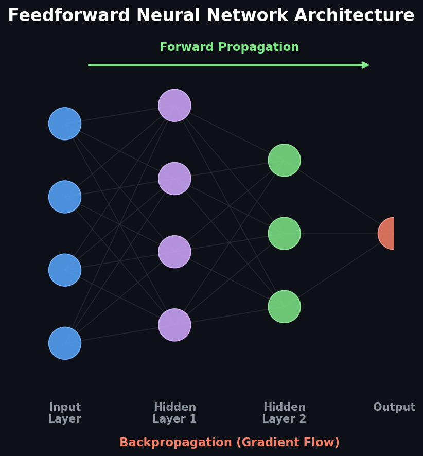
Backpropagation — The Engine of Deep Learning

This was the topic I was most excited about, and the lecture didn't disappoint. Here's how I'd explain backpropagation to my past self:

The Core Idea

You have a neural network that makes a prediction. You compute how wrong that prediction is (the loss). Now you need to figure out: how should I adjust each weight in the network to reduce this loss?

The answer is the gradient of the loss with respect to every weight. Backpropagation is just the chain rule of calculus, applied recursively through the computational graph.

Computational Graphs — The Real MVP

The insight that changed everything for me: any computation can be represented as a directed graph where nodes are variables and edges are operations. Forward propagation pushes values from input to output. Backpropagation pushes gradients from output back to input.

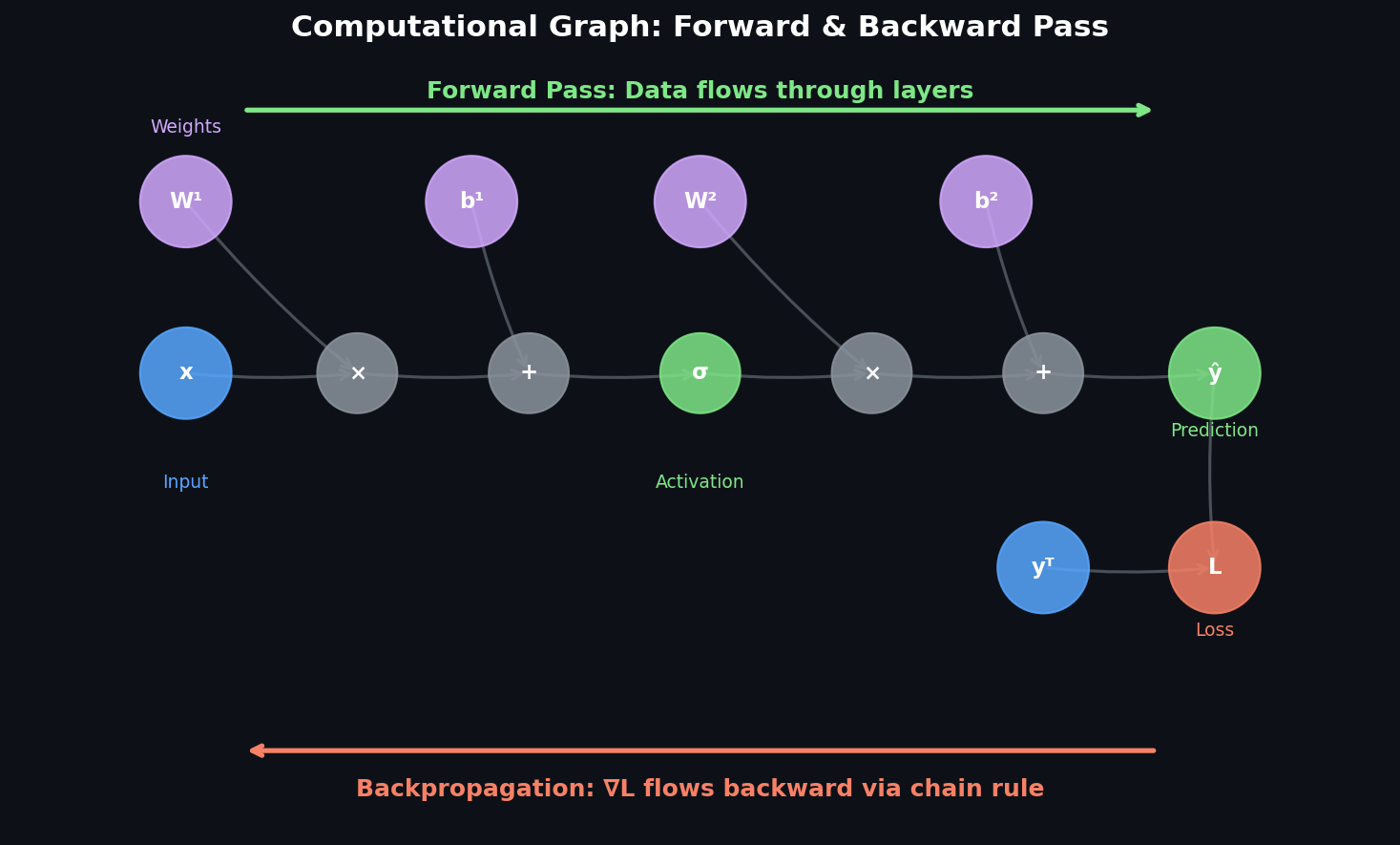
What makes this powerful is that each node only needs to know its local derivative — how its output changes with respect to its inputs. The chain rule handles the rest by multiplying these local derivatives along every path from the loss back to each parameter.

From Exponential to Linear

Without the graph structure, computing gradients would be exponential in the depth of the network — you'd recompute shared sub-expressions over and over. The computational graph approach reduces this to linear time by caching intermediate results (this is the "table-filling" aspect of backprop that's similar to dynamic programming).

Here's the simplified mental model:

• Forward pass: Compute and cache every intermediate value

• Backward pass: Starting from the loss, multiply the incoming gradient by the local Jacobian at each node, pass it downstream

The Jacobian Connection

For vector-valued functions (which is basically every layer), the chain rule involves Jacobian matrices — matrices of partial derivatives. The gradient of the loss with respect to any hidden layer is computed as:

∇_x L = J^T · ∇_y L

This is the Jacobian of the layer's function, transposed, times the gradient flowing back from the next layer. Once you see this, the entire backprop algorithm becomes a sequence of matrix-vector products — which is why GPUs are so effective for training.

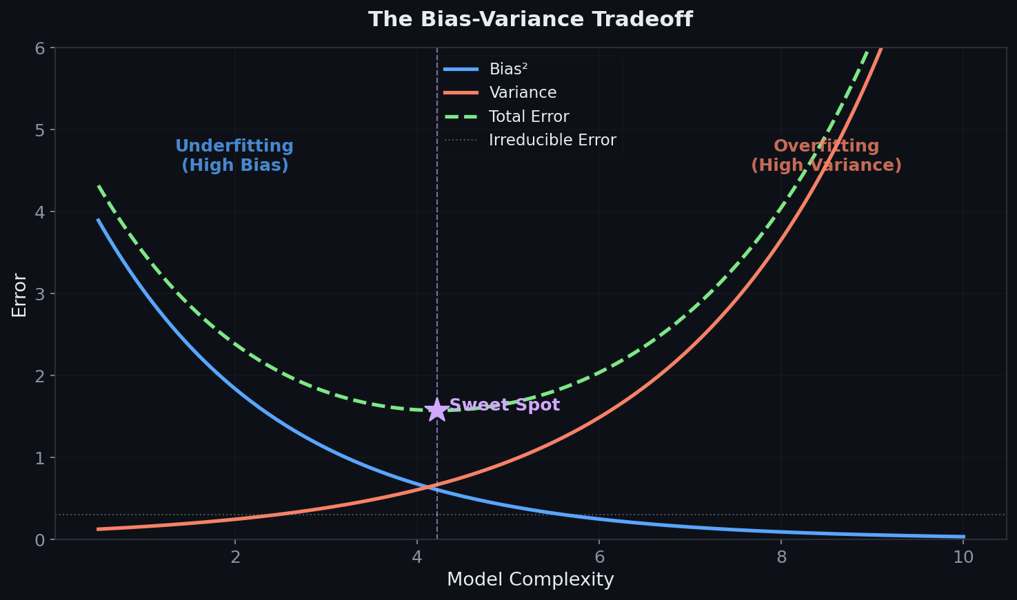
Regularization — Learning to Generalize

One of the most practical topics covered was regularization. The core tension in ML is always memorization vs. generalization — you want your model to learn patterns, not memorize training data.

The regularized loss function looks like:

J(θ) = L(y, ŷ) + λΩ(θ)

Where the first term measures prediction error and the second penalizes model complexity. The key insight: regularization isn't just a trick; it's encoding your prior belief that simpler models are more likely to be correct (Ockham's Razor, formalized).

Key Takeaways So Far

After three weeks of foundations, here's what I've internalized:

1. The math isn't optional. Every debugging session in deep learning eventually comes down to understanding gradients, distributions, or numerical stability. You can get by without it, but you can't get good without it.

2. Everything is optimization. Whether it's regression, classification, or training GPT-4, the paradigm is the same: define a loss, compute the gradient, take a step. The elegance of this unifying framework is underappreciated.

3. Backpropagation is simple but profound. It's just the chain rule. But the way it leverages computational graphs to make gradient computation efficient is a masterclass in algorithm design.

4. Regularization is about beliefs, not just performance. When you add an L2 penalty, you're saying "I believe the true function has small weights." When you use L1, you're saying "I believe most features are irrelevant." These aren't arbitrary choices — they're assumptions about the world.

5. Information theory gives loss functions meaning. Cross-entropy isn't just a function that works — it's the mathematically principled way to measure the difference between what your model believes and what's actually true.

What's Next

The course is just getting started. Coming up: multilayer perceptrons with various architectures, convolutional neural networks for computer vision, sequence models (RNNs, LSTMs, Transformers), generative models, LLMs, and deep reinforcement learning. I'm particularly excited about the Transformer and LLM sections, given how much they've reshaped the field.

I'll keep documenting my journey as the semester progresses. If you're studying these topics or building ML systems in production, I hope these insights help bridge the gap between "I know how to use it" and "I understand why it works."

This is Part 1 of my Neural Networks & Deep Learning series at GWU. Follow along on my Zero to One blog for more.

If you found this helpful, drop a like or reach out — I love connecting with fellow ML engineers and researchers.